An Overview of Differential Privacy in the 2020 Decennial Census
To protect respondents’ privacy, for the 2020 Decennial Census the Census Bureau is using a modern disclosure avoidance approach called differential privacy. In brief, differential privacy adds statistical noise—small random additions or subtractions—into the data to reduce the risk that someone could reidentify any person or household.
Although the Census Bureau has previously used a variety of disclosure avoidance methods to protect respondents’ privacy in decennial censuses, differential privacy is a far more sophisticated approach that is necessary to address the data reidentification threats posed by modern computing capabilities. To learn more about why the Census Bureau is using differential privacy for the 2020 Census, see the Census Bureau’s publication “Why the Census Bureau Chose Differential Privacy.” This video, created in collaboration with the Census Bureau, provides a helpful introduction to why differential privacy is necessary and how it works.
Differential privacy was applied both to the Redistricting Data that were released in August of 2021 and to the more detailed Demographic and Housing Characteristics (DHC) File that was released on May 25th, 2023. The DHC file includes detailed tables on age, sex, race, Hispanic or Latino origin, household and family types, group quarters populations, housing occupancy, and housing tenure (owning versus renting) down to the census block level.
When the 2020 DHC file was released, the Census Bureau also released summary metrics for the amount of error introduced to data for selected types of geographies and populations by the disclosure avoidance system. Although noise was introduced by disclosure avoidance approaches in prior decennial censuses, this is the first decennial census for which the Census Bureau has published metrics quantifying this noise.
In this post, we will: (1) describe how differential privacy is applied to the 2020 Decennial Census data; (2) review the Census Bureau’s guidance for 2020 Decennial Census data users; (3) provide an overview of the summary metrics file released by the Census Bureau; and (4) discuss some illustrative examples of the amount of error introduced to certain counts as reported in the summary metrics file.
How is Differential Privacy Applied to the 2020 Decennial Census?
Differential privacy is applied to the 2020 Decennial Census in a multi-step process referred to as the TopDown Algorithm. First, differentially private algorithms are used to inject statistical noise into the cells of all possible cross-tabulations in the 2020 Decennial Census tables. The Census Bureau then post-processes these noisy data to improve internal consistency in a series of steps from higher to lower levels of geography. For more technical details, see the Census Bureau’s publications “Disclosure Avoidance for the 2020 Census: An Introduction” and “Disclosure Avoidance and the 2020 Census: How the TopDown Algorithm Works.”
Two factors that influence how much noise is added to any given count (that is, the number of people or housing units with particular combinations of characteristics, for example the number of Black or African American children under 1 year old in Hartford) are:
The amount of the “privacy-loss budget” that is allocated to that count
The distance of the geography for the count (for example, if the count is for a school district or town) from the “geographic spine” used in the Top-Down Algorithm
We will discuss both concepts below. In addition, all users should keep in mind that counts for small geographies (for example, census blocks and tracts) and for small populations will have more relative noise added by differential privacy (that is, the amount of noise as a proportion of the population size) than do counts for larger geographies and populations.
The Privacy-Loss Budget
The Census Bureau is seeking to balance the usefulness of the data with the protection of privacy. On one side of the scale is complete usefulness to people using the data to make decisions and no protection of privacy (complete accuracy). The other side of the scale is complete privacy protection with no usefulness (no accuracy). Differential privacy seeks to balance these two competing priorities with the privacy-loss budget.
The privacy-loss budget quantifies the maximum disclosure risk of the publicly released data. Higher privacy-loss budgets yield more accurate counts (more usefulness) with lower privacy protection, whereas lower privacy-loss budgets yield less accurate counts (less usefulness) with higher privacy protection.
The Census Bureau allocates a proportion of the overall privacy-loss budget to each geographic level (from the nation down to census blocks – see more below) and to each “query” within each geographic level (for example, Hispanic ethnicity by race) that is used to produce the published tables. The proportion of the privacy-loss budget that is allocated to each query within each geographic level controls the amount of noise that is likely to be injected into each published count. Counts for geographies and queries with a higher privacy-loss budget allocation will have higher accuracy.
Decisions about how accurate a given count should be depend on assessments of how important it is for the count to be highly accurate and how likely it is that an accurate count will increase the risk of reidentification. For example, a count of the number of people in Connecticut who are of Hispanic ethnicity could be highly accurate without high reidentification risk because it is calculated across the entire state. However, a highly accurate count of the number of people living in a given census tract in Hartford who are 65 years old and of Hispanic ethnicity would come with a much higher reidentification risk and therefore needs more protection.
The Census Bureau has fine-tuned the privacy-loss budget allocations based on both internal analyses and user feedback on the data’s fitness-for-use. However, the allocations necessarily reflect the Census Bureau’s prioritization of many competing use cases for the data (that is, how important it is for each count to be accurate).
Geographies and the “Geographic Spine”
Decennial census data are information about people and housing in specific places, and these places are called “geographies.” The “geographic spine” is a hierarchy of nested geographies used in Census Bureau data products, shown in the graphic below (the line down the middle from Nation to Census Blocks).

Source: U.S. Census Bureau. “Disclosure Avoidance and the 2020 Census: How the TopDown Algorithm Works”
The TopDown Algorithm is applied to a modified version of this geographic hierarchy. We will describe these modifications below, but first there are two important things to know about the geographic spine as it relates to the noise introduced by differential privacy:
Counts for off-spine geographies have more absolute noise (that is, a greater mean absolute error) than do counts for on-spine geographies. This is because counts for off-spine geographies are calculated by combining (adding or subtracting) the counts for on-spine geographies. When the counts are combined in this way, the noise injected by differential privacy accumulates in the off-spine geographies.
Connecticut’s towns and cities are an off-spine geography, which means they will have more noise in their counts than do on-spine geographies.
In response to user feedback, the Census Bureau modified the geographic hierarchy used in the TopDown Algorithm to reduce the amount of noise in key off-spine geographies. Specifically, the Census Bureau processed all American Indian, Alaska Native, and Native Hawaiian Areas separately to increase the accuracy of counts within these areas, and they created “optimized block groups” to more closely align with the borders of census designated places and minor civil divisions.
For Connecticut, these optimized block groups should reduce the amount of noise injected into counts for our towns and cities. Additionally, for the detailed demographic characteristics reported in the DHC (but not the Redistricting Data), the Census Bureau further modified the geographic hierarchy to incorporate the “Primitive Geographies” used by the Census Bureau’s Population Estimates Program, which should further reduce the noise in detailed demographic estimates for Connecticut’s towns and cities.
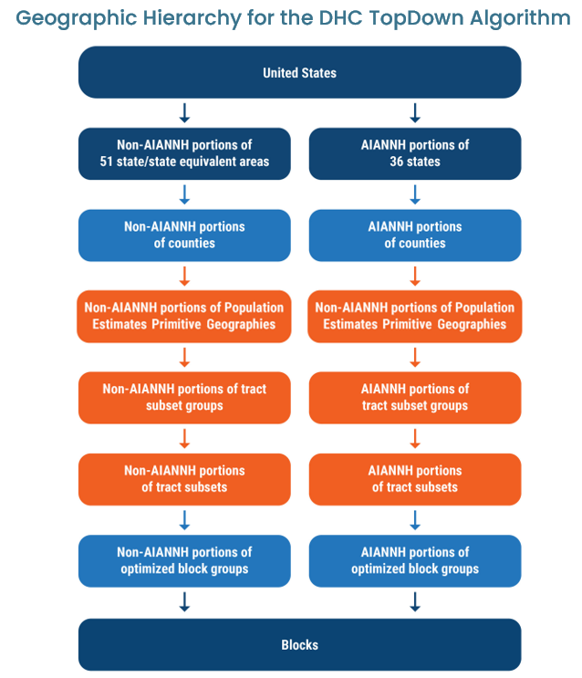
Source: U.S. Census Bureau. “Disclosure Avoidance and the 2020 Census: How the TopDown Algorithm Works”
Post-Processing
After noise is added to the data at each level of the geographic hierarchy, the Census Bureau conducts a series of post-processing steps that apply certain non-random constraints to the noisy data. Specifically, the following counts were constrained to equal the enumerated census counts with no noise added (that is, they were held “invariant”). Simply put, these counts did not have differential privacy applied to them and they match the numbers in the confidential Census Edited File, which is the original census response data edited for quality (e.g., filling in missing values):
The total number of people in each state, the District of Columbia, and Puerto Rico
The total number of housing units (but not population counts) for all geographic levels
The number of occupied group quarters facilities (but not population counts) in each census block by the type of group quarters (e.g., correctional facilities, nursing homes, college student housing, etc.)
Additionally, certain constraints were applied at all nesting geographic levels to improve the reasonableness and internal consistency of the results. These include:
Population and housing unit counts were constrained to be non-negative integers.
Population-related counts were constrained to be consistent within tables, across tables, and across geographies. For example, the sum of the population in each age group must equal the total population, and the sum of the population in each county within a state must equal the state’s total population.
Housing-related counts were constrained to be consistent within tables, across tables, and across geographies. For example, the number of occupied and vacant housing units must sum to the total number of housing units, and the number of vacant housing units in each county within a state must sum to the state’s total number of vacant housing units.
Counts in the DHC tables were constrained to be consistent with the previously-released Redistricting Data.
Although the noise injection step of the TopDown Algorithm results in noisy but unbiased data (meaning the noise is random and averages to zero), the post-processing steps introduce some biases in the data. By biases, we that the published counts for certain types of populations or geographies are higher or lower than the enumerated data. For example, small populations tend to have positively biased counts because of the constraint that all counts must be non-negative integers.
Census Bureau Guidance for Data Users
By design to protect respondents’ privacy, lower levels of geography and smaller populations contain more relative noise (that is, the amount of error as a percentage of the population or housing unit count) than do higher levels of geography or larger populations. For this reason, the Census Bureau advises that block-level and small-population data may be inaccurate and should be aggregated before use. Aggregating smaller geographies or populations yields smaller relative errors even if the absolute error is greater and/or the aggregation yields an off-spine geography.
Since counts were not constrained to be consistent across the population-related and housing-related tables, the Census Bureau advises against dividing across the person and household tables at low levels of geography (e.g., tracts or lower), as this may yield improbable results. For example, calculating the average number of persons per household in a census block by dividing the number of people in households (population data) by the number of occupied housing units (housing data) could yield more occupied housing units than people, or blocks with people but no occupied housing units (see the Census Bureau’s publication “Disclosure Avoidance for the 2020 Census: An Introduction” and the 2020 Census Impossible Blocks Viewer by Georgetown University’s Massive Data Institute).
Understanding Accuracy of the Data: 2020 DHC Summary Metrics
Along with the 2020 DHC file, the Census Bureau released summary metrics for the amount of error injected into certain types of counts by the disclosure avoidance system. Specifically, they released:
Mean absolute error, which shows how close the published data point is to the enumerated count on average (i.e., the accuracy of the count).
Mean error, which shows whether the published data point tends to go higher or lower than the enumerated count and by how much (i.e., bias in the count).
Below, we discuss some illustrative examples of mean absolute errors in 2020 Decennial Census population counts as reported in the Census Bureau’s summary metrics.
Mean Absolute Error in County-Level Total Population Counts
Since counties are on the geographic hierarchy used in the disclosure avoidance system, mean absolute errors for total population at the county level are very small regardless of the size of the county.
Averaged across all counties in the United States, the mean absolute error for county-level total populations is about 2 people regardless of the size of the county.
Mean Absolute Error in Minor Civil Division Total Population Counts (including CT’s towns)
In contrast, since minor civil divisions (including Connecticut’s towns) are not on the geographic hierarchy used in the disclosure avoidance system, mean absolute errors grow as the size of the minor civil division increases. This presumably reflects the greater number of on-spine geographies that must be combined to generate counts for larger minor civil divisions.
Although these mean absolute errors are larger than what was seen for counties, they are still small - a difference of about 2 people on average for minor civil divisions with populations under 1,000 and about 9.5 people on average for minor civil divisions with populations over 50,000.
It is important to note that the relative error (that is, error as a proportion of the population) should always decrease as the population size increases. Unfortunately, the Census Bureau has not yet released summary metrics for relative error. However, we can get a sense for this by calculating that the relative error for 2 people out of 1,000 is 0.2% whereas the relative error for 9.5 people out of 50,000 is 0.02%.
Mean Absolute Error in Unified School District Total Population Counts
Mean absolute errors for the total population within unified school districts, on the other hand, are substantially larger than those for similarly sized minor civil divisions. For example, across the United States, school districts with a total population of 10,000 - 49,999 have a mean absolute error of 28.5 people, versus 4.4 people for similarly sized minor civil divisions.
Still, these mean absolute errors are fairly small (for example, 28.5 people out of 10,000 would be a relative error of 0.3%). As with any other geography, the relative error will decrease as the population increases even though the mean absolute error becomes greater.
Mean Absolute Error in Unified School District Population Counts by Year of Age
Counts by single year of age for children and youth within all unified school districts in the U.S. have a mean absolute error of about 5 individuals within each year of age. Again, it is important to keep in mind that the relative error will be larger for smaller school districts. Additionally, combining age groups should decrease the relative error in the count since the population size will be larger.
More Details Available in the Summary Metrics File
The charts above illustrate just a few examples of what is available in the summary metrics file. The summary metrics file includes mean absolute errors and mean errors for selected counts in both the 2020 Decennial Census population and housing data files. For the population data, these include:
Total population within counties, incorporated places, census tracts, minor civil divisions (which include Connecticut’s towns), and school districts
Race, Hispanic ethnicity, and age by sex within states, counties, incorporated places, and census tracts (but not minor civil divisions)
Single year of age for children and youth in counties and school districts
For the housing data, these include:
Counts of occupied units within counties, incorporated places, census tracts, minor civil divisions, and school districts
Tenure (owner or renter) by race, age, and Hispanic ethnicity of householder within states, counties, incorporated places, and census tracts (but not minor civil divisions)
Household type and size within states, counties, incorporated places, school districts, and census tracts (but not minor civil divisions)
We encourage interested readers to explore the summary metrics with their own use cases in mind.
More Details to be Released on 2020 Decennial Census Data Accuracy
Since the differential privacy summary metrics shared by the Census Bureau are averages, they do not tell us how much error is introduced to the count for any particular geography or population within that geography. Variability around these averages can have important implications for local decision-making using census data. Moreover, summary metrics are not provided for all geographies or characteristics in the DHC.
The Census Bureau is planning on releasing more detailed metrics in the future including average percent error (i.e., the amount of error relative to the population size) and counts of outliers, as well as confidence intervals for the published counts. However, they have not yet released a timeline for these products (see the Census Bureau’s blog post “What to Expect: Disclosure Avoidance and the 2020 Census Demographic and Housing Characteristics File”).
The Census Bureau has released in-depth demonstration data products to allow data users to analyze the likely impacts of differential privacy on the accuracy of specific counts. We plan to share a data tool and blog post using these products to explore the likely impact of differential privacy on Connecticut’s 2020 Decennial Census counts in the future. Make sure you’re signed up for our newsletter to be notified when this is released!
For More Information
To learn more about differential privacy and the 2020 Decennial Census, you can explore CTData’s Differential Privacy page and the Census Bureau’s page on Understanding Differential Privacy. Here are some additional resources:
Protecting Privacy with Math (video)
Disclosure Avoidance and the 2020 Census: How the TopDown Algorithm Works
Implementing Differential Privacy: Seven Lessons From the 2020 United States Census
Check out our Event Calendar for census-related events.
If you are interested in learning more about CTData, check out our mission and values and the services we provide. For training and tips on how to use data to inform your personal and professional life, register for one of our CTData Academy workshops or browse our blog. You can keep up with us by subscribing to the CTData newsletter and following us on Twitter, Facebook, and LinkedIn.